InternVL 3.5

Brief intro

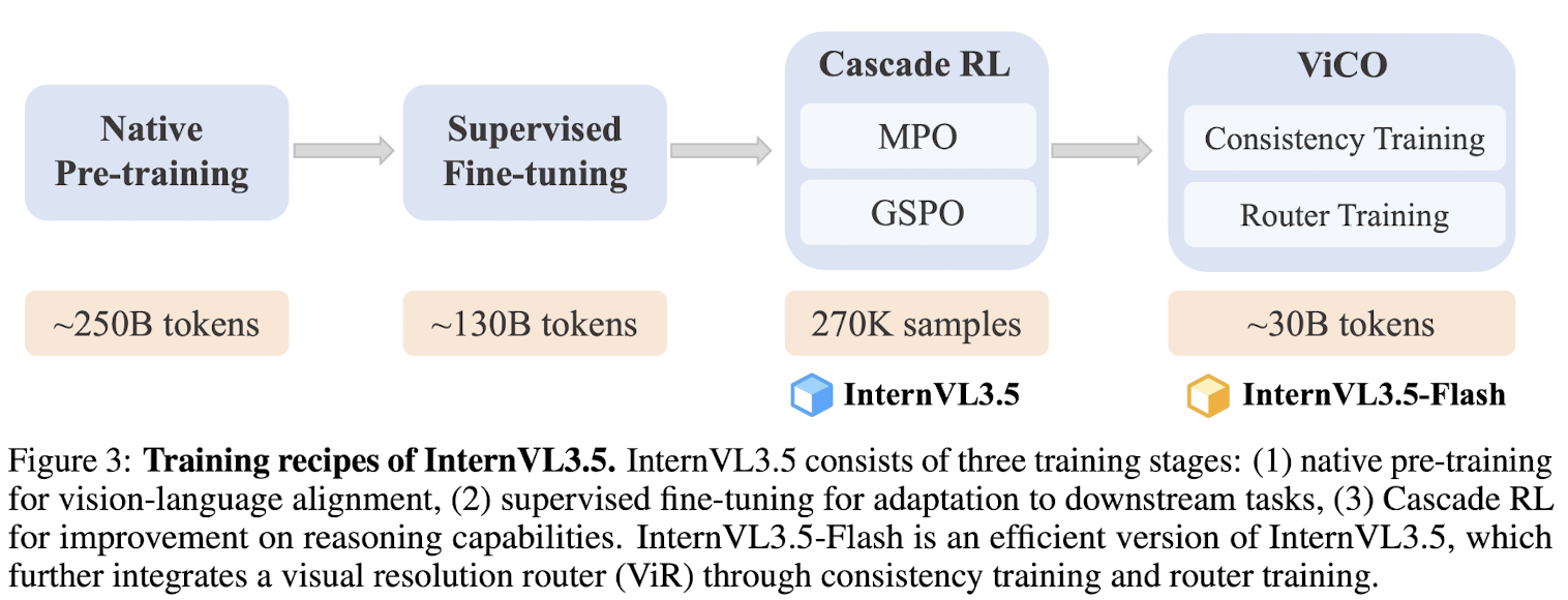
Cascade RL introduced in InternVL3.5, which enhances reasoning through a two-stage process:

• offline RL for stable convergence, efficiently achieves satisfactory performance
• online RL for refined alignment, carefully refines the output distribution and further push the performance upper bound of the model

A Visual Resolution Router(ViR) that dynamically adjusts the resolution of visual tokens without compromising performance helps optimizing efficiency.

• aims to dynamically select the best trade-off resolution of visual tokens, reducing the inference costs with a negligible performance sacrifice
• ViR can be efficiently integrated into InternVL3.5 with a light training stage namely Visual Consistency Learning(ViCO).

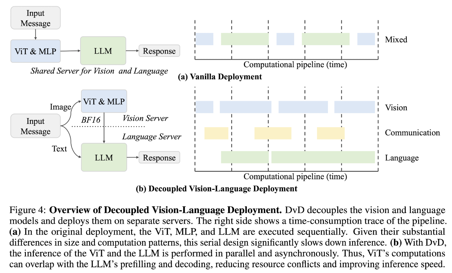
The Decoupled Vision-Language Deployment(DvD) strategy separates the vision encoder and language model across different GPUs, effectively balancing computational load.

Model Architecture

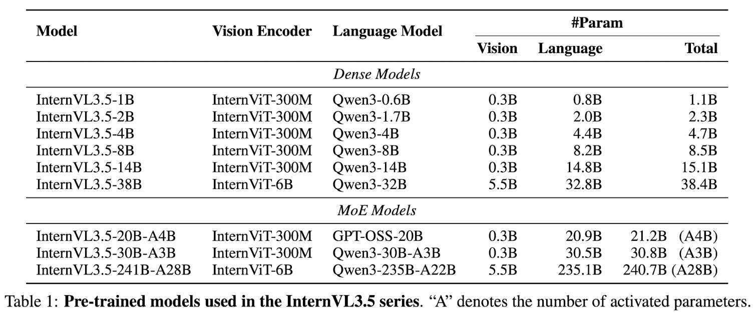
The InternVL3.5 follows ViT-MLP-LLM paradigm

• Qwen3 series and GPT-OSS as LLM
• InternViT-300M and InternViT-6B as vision encoder
• each image patch is initially represented as 1024 visual tokens for vision encoder, then compressed into 256 tokens via a pixel shuffle module to LLM
• Dynamic High Resolution, to improve image understanding at varying resolutions

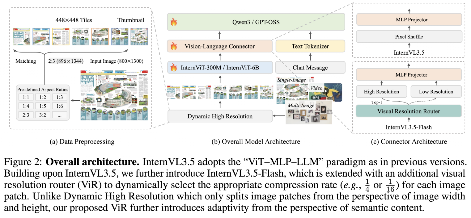The InternVL3.5-Flash

• integrates the Visual Resolution Router(ViR), yielding a series of efficient variants suitable for resource-constrained scenarios.
• an additional pixel shuffle module with a higher compression rate to compress the visual tokens down to 64 tokens
• the patch router determines the appropriate compression rate by assessing the semantic richness of each patch

Pre-Training

Update all model params jointly using the combination of large-scale text and multimodal corpora.

Given an training sample of multimodal token sequence $x=(x_{1},x_{2},..,x_{L})$, the next token prediction(NTP) loss is calculated on each text token(真正算 loss 的只在 text tokens 上):

$$\mathcal{L}_{i}=-\log p_{\theta}(x_{i}|x_{1},\dots,x_{i-1})$$

the predicted token or prefix tokens can be either text or image tokens.

only response tokens are calculated in conversation samples

Adopt the square averaging to re-weight the NTP loss to mitigate bias toward either longer or shorter responses during training

$$\mathcal{L}_{i}'=\frac{w_{i}}{\sum_{j}w_{j}}\cdot \mathcal{L}_{i},\quad w_{i}=\frac{1}{N^{0.5}}$$

where $N$ is the number of tokens in the training sample on which the loss needs to be calculated.

Data.

• multimodal data
• text-only data
• max sequence length is 32K

Post-Training

Three stage post-training strategy:

• SFT: use high-quality conversation data to further enhance the model's capability
• Cascade RL
• Visual Consistency Learning(ViCO): aims to integrate visual resolution router(ViR) into InternVL3.5 to construct Flash model, by minimizing the output divergence of different visual compression rates

SFT

• same objective and square averaging strategy to calculate final loss
• context window 32K to adapt long-context information
• instruction-following data, multimodal reasoning data, capability-expansion datasets

Cascade RL

1. First finetune the model using an offline RL algorithm as an efficient warm-up stage to reach satisfied results, and guarantee high-quality rollouts latter.
2. Employ an online RL algorithm to further refine the output distribution based on rollouts generated by the model itself.

Offline RL Stage Employ mixed preference optimization(MPO) to finetune the model. The training objective of MPO combines

• preference loss $\mathcal{L}_{p}$ (the DPO loss),
• quality loss $\mathcal{L}_{q}$ (the BCO loss),
• and generation loss $\mathcal{L}_{g}$ (the LM loss):

$$\mathcal{L}_{\text{MPO}}=w_{p}\mathcal{L}_{p}+w_{q}\mathcal{L}_{q}+w_{g}\mathcal{L}_{g}$$

Online RL Stage Employ GSPO, without reference model constraints as online RL algorithm. The advantage is defined as the normalized reward across responses sampled from the same query:

$$\hat{A}_{i}=\frac{r(x,y_{i})-\text{mean}\bigg(\{r(x,y_{i}\}_{i=1}^G\bigg)}{\text{std}\bigg(\{r(x,y_{i}\}_{i=1}^G\bigg)}$$

• $y_{i}$ is the $i$-th response generated for the query $x$
• $G$ is the total number of generated responses to the query
• $r(x,y_{i})$ denotes the reward for this response

The training objective is

$$\mathcal{L}_{\text{GSPO}}(\theta)=\mathbb{E}_{x\sim\mathcal{D}, \{y_{i}\}_{i=1}^G\sim \pi_{\theta_{\text{old}}}(\cdot|x)}\left[ \frac{1}{G}\sum_{i=1}^G \min\left(s_{i}(\theta)\hat{A}_{i}, \text{clip}(s_{i}(\theta), 1-\epsilon,1+\epsilon)\hat{A}_{i}\right) \right]$$

the importance sampling ratio is defined as the geometric mean of the per-token ratios:

$$s_{i}(\theta)=\left( \frac{\pi_{\theta}(y_{i}|x)}{\pi_{\theta_{\text{old}}}(y_{i}|x)} \right)^{1/|y_{i}|}=\exp\left( \frac{1}{|y_{i}|}\sum_{t=1}^{|y_{i}|}\log \frac{\pi_{\theta}(y_{i,t}|x,y_{i,<t})}{\pi_{\theta_{\text{old}}}(y_{i,t}|x,y_{i,<t})} \right)$$

where $\pi_{\theta}(y_{i}|x,y_{i,<t})$ and $\pi_{\theta}(y_{i,t}|x,y_{i,<t})$ denote the generation probability of response $y_{i}$ and token $y_{i,t}$ under the policy model with parameters $\theta$.

Cascade RL Advantage

• more stable：离线阶段解耦 rollout 收集与参数更新，有效缓解奖励噪声等问题；在线阶段中，更强的初始模型表现出更稳定的训练动态，MPO 阶段的性能增益进一步提升了 GSPO 阶段的鲁棒性。
• more efficient：MPO 阶段的 rollout 可跨模型共享，摊薄在线 RL 的采样成本。
• higher performance ceiling：经 MPO 微调的模型在后续在线 RL 阶段以更少训练步数达到更高性能，显著降低总体训练开销。

Visual Consistency Learning

ViCO helps reducing the inference cost of InternVL3.5, termed as InternVl3.5-Flash. ViCO comprises two stages:

Consistency training The entire model is trained to minimize the divergence between response distributions conditioned on visual tokens with different compression rates.

ViCO需要解决：当图像被更 aggressively 压缩成更少的 visual tokens 时，让模型输出的 token 分布尽量和「高质量视觉输入」时的一样。 实际上就是 视觉压缩下的「分布对齐」蒸馏。用 KL distillation 让 “低视觉分辨率版本的 InternVL3.5”（policy）在任何给定文本前缀下，对下一个 token 的分布尽量逼近 “高视觉分辨率版本的 InternVL3.5”（reference）。

An extra reference model(frozen and initialized as InternVL3.5) is introduced in practices. Each image patch is represented as either 256 or 64 tokens, and the training objective is

$$\mathcal{L}_{\text{ViCO}}=\mathbb{E}_{\xi \sim \mathcal{R}}\left[ \frac{1}{N} \sum_{i=1}^N\text{KL}\bigg(\pi_{\theta_{ref}}(y_{i}|y_{<i},I)\bigg\Vert\pi_{\theta_{policy}}(y_{i}|y_{<i},I_{\xi})\bigg)\right]$$

where $\xi \sim \mathrm{Unif}\!\left\{ \tfrac14, \tfrac1{16} \right\}$ represents the compression rate. The image $I_{\xi}$ represents 256 tokens when $\xi=\frac{1}{4}$ and 64 tokens when $\xi=\frac{1}{16}$.

The reference model always performs with $\xi=\frac{1}{4}$.

这个 reference model 可以被视为一个 teacher model，它用于看高质量视觉表示，即256 tokens。

Router training Train the ViR to select an appropriate trade-off resolution for different inputs. ViR is formulated as a binary classifier and trained using standard cross-entropy loss.

Stage 2 在 Stage 1 的基础上，冻结模型的主干权重，训练一个 ViR 二分类器，用来判断每个图像 patch 是否可以压缩以节省算力，还是得保留原分辨率来保证质量。

First compute the KL divergence between the model outputs conditioned on uncompressed visual tokens(256 tokens/patch) and those conditioned on compressed visual tokens(64 tokens/patch). The main MLLM(ViT, MLP, LLM) kept frozen, only ViR is trained.

The loss ratio for each patch:

$$r_{i} = \frac{\mathcal{L}_{\text{ViCO}}\left( y_{i}|I_{\frac{1}{16}} \right)}{\mathcal{L}_{\text{ViCO}}\left( y_{i}|I_{\frac{1}{4}} \right)}$$

the ratio quantifies the relative increase in loss caused by compressing the visual tokens.

The binary ground-truth label for the patch router based on the ratio is:

$$y_{i}^{\text{router}}=\begin{cases} 0,\quad r_{i}<\tau~\text{(compression has negligible impact)}, \\ 1,\quad r_{i}>\tau~\text{(compression has significant impact)} \end{cases}$$

where $y_{i}^\text{router}=0~\text{when}~\xi=\frac{1}{16}$ and $y_{i}^\text{router}=1~\text{when}~\xi=\frac{1}{4}$.

ViR 输出一个二元标签，$0$ 则可以压缩(64 tokens)，1则保留高分辨率(256 tokens)。给到 ViR 的标签由 看压缩前后 ViCO loss 的变化幅度 来决定。 如果 $r_i \approx 1$：压缩前后 loss 差不多 → 压缩几乎不伤性能 → 这个 patch 对压缩不敏感；如果 $r_i \gg 1$：压缩后 loss 明显变大 → 压缩伤害很大 → 这个 patch 很敏感，需要高分辨率保真。

During training, the historical $r_i$ values of a sliding window are stored, and $\tau$ is a dynamical threshold computed from the $k$-th percentile of historical $r_{i}$ values.

在训练过程中，他们维持一个滑动窗口，里面存最近一段时间的 $r_i$​ 值；然后把 $\tau$ 定义成这些历史 $r_i$ 的 第 $k$ 个百分位数(k-th percentile)。如：如果 $k=80$，那么 $\tau$ 就是「80% 样本的 $r_i$​ 都小于它」的那个值。

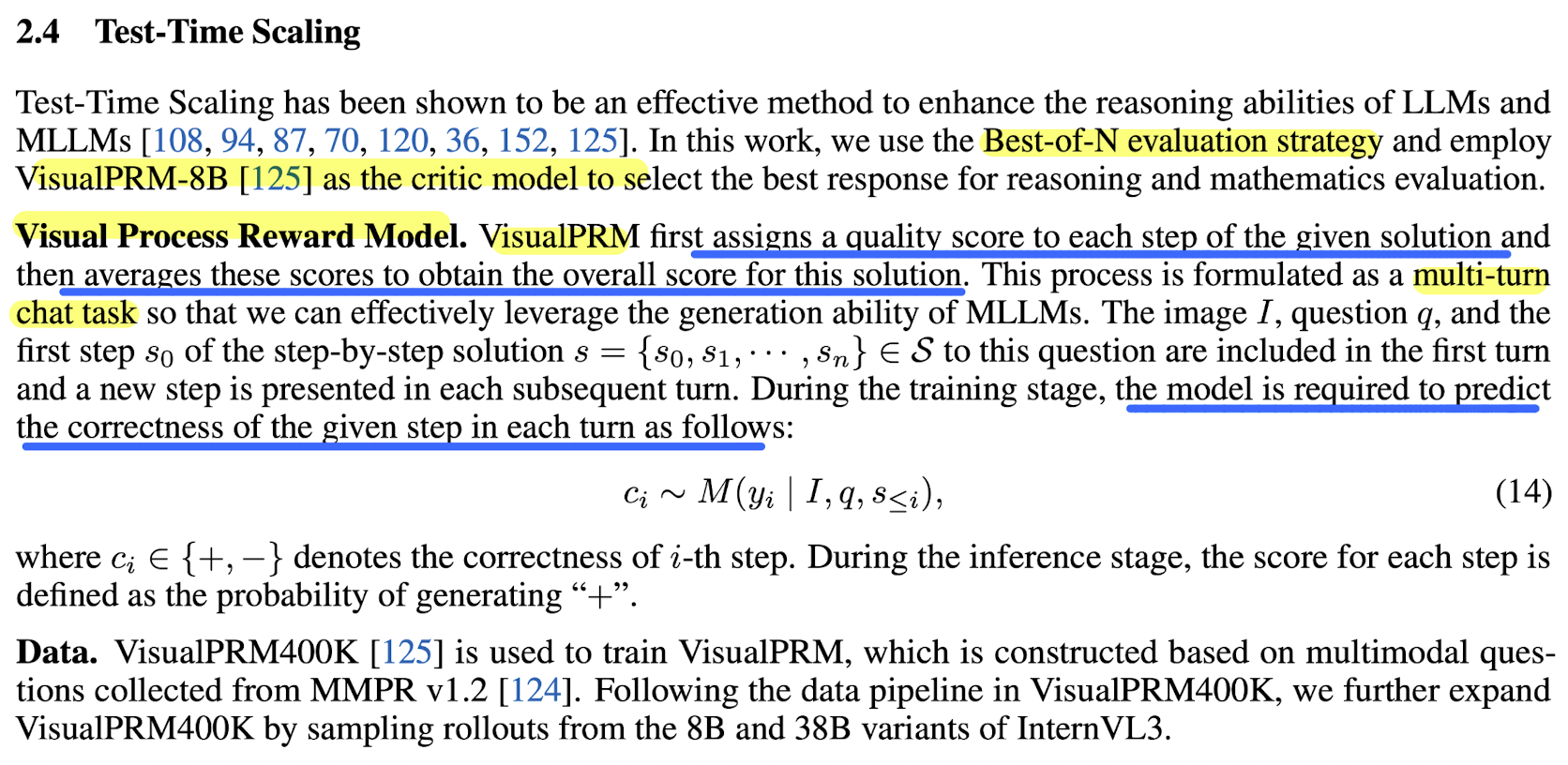
Test-Time Scaling

Deep Thinking Guide the model to deliberately engage in step-by-step reasoning. Parallel Thinking Adopt the Best-of-N(BON) strategy by employing VisualPRM-v1.1 as the critic model to select the optimal response from multiple reasoning candidates.

Infrastructure

Decoupled Vision-Language Deployment(DVD) DVD separates vision and language processing, with a particular focus on optimizing the pre-filling stage.

The ViT and MLP(and ViR) are deployed on the vision server, while the LLM is deployed on the language server. The visual patches are batched and processed to produce the compact feature embeddings in vision server, and then transmitted to the language server for fusion with text prior to decoding. The communication is unidirectional, the BF16 visual features is transmitted over TCP.

InternVL3

Model Architecture

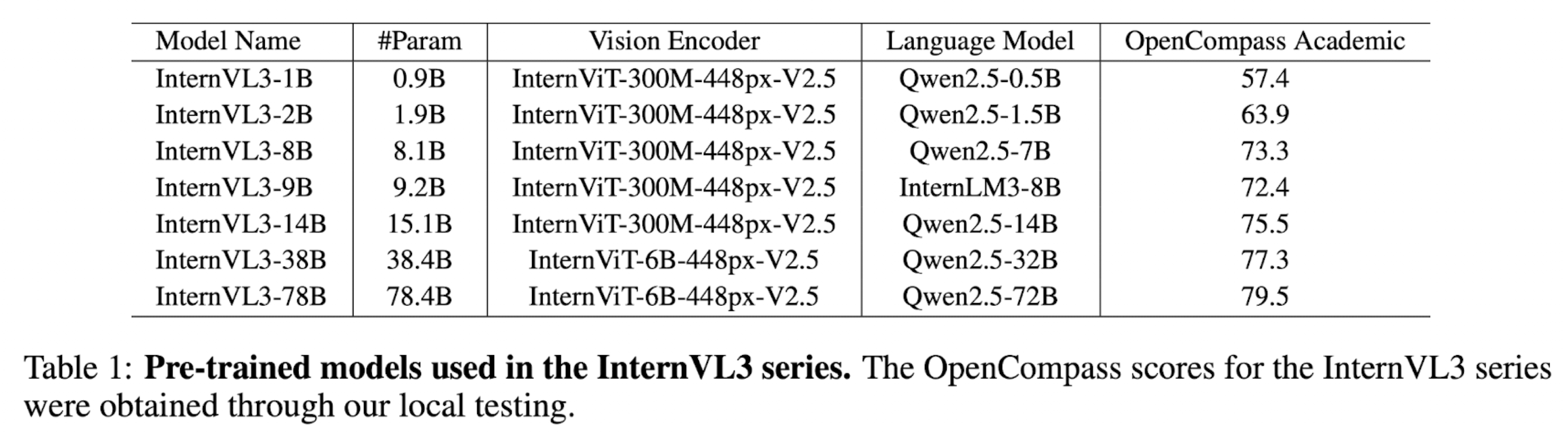The InternVL3 follows ViT-MLP-LLM paradigm

• initialize ViT and LLM from pretrained model weights
• vision encoder: InternViT-300M and InternViT-6B
• LLM: Qwen2.5 and InternLM3-8B
• MLP: 2 layer network with random initialization
• pixel unshuffle operation to enhance scalability for processing high-resolution images and reduces the visual token count to $\frac{1}{4}$ of its origin, representing each $448\times448$ image tile with 256 visual tokens.

Variable Visual Positional Encoding(V2PE)

V2PE uses smaller, more flexible position increments for visual tokens. It handles the longer multimodal context without excessively extending the position window.

The position index $p_{i}$ for any token $x_{i}\in x,~x=(x_{1},\dots ,x_{L})$ can be sequentially computed as

$$p_{i}=\begin{cases} 0,\quad\text{if }i=1 \\ f_{\text{pos}}(p_{i-1},x_i)\quad\text{for }i=2,3,\dots,N \end{cases}$$

V2PE employs a modality-specific recursive function for position index computation.

$$p_{i}=p_{i-1}+\begin{cases} 1,\quad\text{if }x_{i}\text{ is a textual token} \\ \delta,\quad\text{if }x_{i}\text{ is a visual token} \end{cases}$$

where $\delta<1$ is a smaller increment, reducing the rate at which position indices increase for visual tokens.

V2PE 将图像的「位置跨度」缩短到原本的 $\frac{1}{\delta}$，使整条序列「有效位置长度」大大减小，更不容易超出模型预训练时的 RoPE 窗口。

During training, $\delta$ is randomly chosen for each image from a predefined set of fractional values:

$$\delta \in \Delta=\left\{ 1, \frac{1}{2}, \frac{1}{4}, \frac{1}{8}, \frac{1}{16}, \frac{1}{32}, \frac{1}{64}, \frac{1}{128}, \frac{1}{256}\right\}$$

训练时，对每张图片的 $\delta$ 都是从 $\Delta$ 中随机挑选的一个值，可以理解为一种 位置缩放的数据增强。。

During inference, $\delta$ can be flexibly selected based on the input sequence length, enabling a balance between task performance and ensuring that position indices remain within the model's valid context length.

推理时，根据 输入的总长度 来选 $\delta$。

在一个统一的 RoPE 位置轴上，文字用大步走，图像用小步走，而且小步的步长在训练中就已经被随机化过，推理阶段可以按当前输入的长短自由调节。

Native Multimodal Pre-Training

Native multimodal pre-training consolidates language pre-training and multi-modal alignment training into a single pretraining stage using multimodal data with large-scale textual corpora during the pretraining process. The scheme enables the pretrained model to learn both linguistic and multimodal capabilities simultaneously.

用「多模态样本 + 大规模纯文本」混在一起，统一用 自回归 NTP 目标 预训练整个 ViT-MLP-LLM。

Adopt the standard left-to-right autoregressive objective:

$$\mathcal{L}_{\text{full}}(\theta)=-\sum_{i=2}^Lw_{i}\cdot \log p_{\theta}(x_{i}|x_{1},\dots,x_{i-1})$$

where $w_{i}$ is the loss weight of token $i$. The loss computation is restricted to only the text tokens

$$\mathcal{L}_{\text{text-only}}(\theta)=-\sum_{i=2,~x_{i}\in \text{ Text}}^L w_{i}\cdot \log p_{\theta}(x_{i}|x_{1},\dots,x_{i-1})$$

In this objective, visual tokens serve as conditioning context for text prediction and are not directly predicted. 图像 token 只作为条件上下文，不被预测。Thus, the model learns to embed multimodal information in a manner that is beneficial for downstream language decoding tasks.

The token weight $w_{i}$ adopts square averaging

$$w_{i}=\begin{cases} \frac{1}{l^0},\quad\text{for token averaging} \\ \frac{1}{l^{0.5}},\quad\text{for square averaging} \\ \frac{1}{l^1},\quad\text{for sample averaging} \end{cases}$$

where $l$ is the number of tokens in the training sample on which the loss needs to be calculated.

token/sample averaging leads to gradients biased towards longer and shorter responses respectively

• token averaging：同一条样本里每个 token 权重相同、与长度无关，长样本(长回答)在梯度里占比更大。梯度偏向 长回答
• sample averaging：一条样本所有 token 权重相同但依赖长度，每条样本的总权重一样，不管长短。也就是，短样本里每个 token 的权重大于长样本里的每个 token。梯度偏向 短回答
• square averaging：长样本依然更重要，但优势被开平方削弱；短样本也有存在感，但不会像 sample averaging 那样被过度放大。

Joint Parameter Optimization: updates all model params jointly during multimodal pretraining

$$\theta^\star=\arg\min_{\theta} \mathbb{E}_{x \in \mathcal{D}_{\text{multi}}}[\mathcal{L}_{\text{text-ony}}(\theta)]$$

原生多模态预训练，一步统一地用 text-only 自回归目标在多模态+纯文本数据上 joint 更新 ViT、MLP 和 LLM。优点是语言和视觉能力从预训练开始就深度耦合，避免了多阶段对齐带来的遗忘和 patch 式修补；缺点是对数据比例和训练配置更敏感，同时牺牲了一部分模块化，可复用现成 LLM 的优势。

Post-Training

2 stage post-training strategy to further enhance the multimodal conversation and reasoning abilities.

• SFT: train the model to imitate the high-quality responses under positive supervision signals
• MPO: improve overall abilities

SFT

• random jpeg compression
• square loss re-weighting
• multimodal data packing
• higher-quality and more diverse training data: tool using, 3D scene, GUI operations, long context tasks, etc.

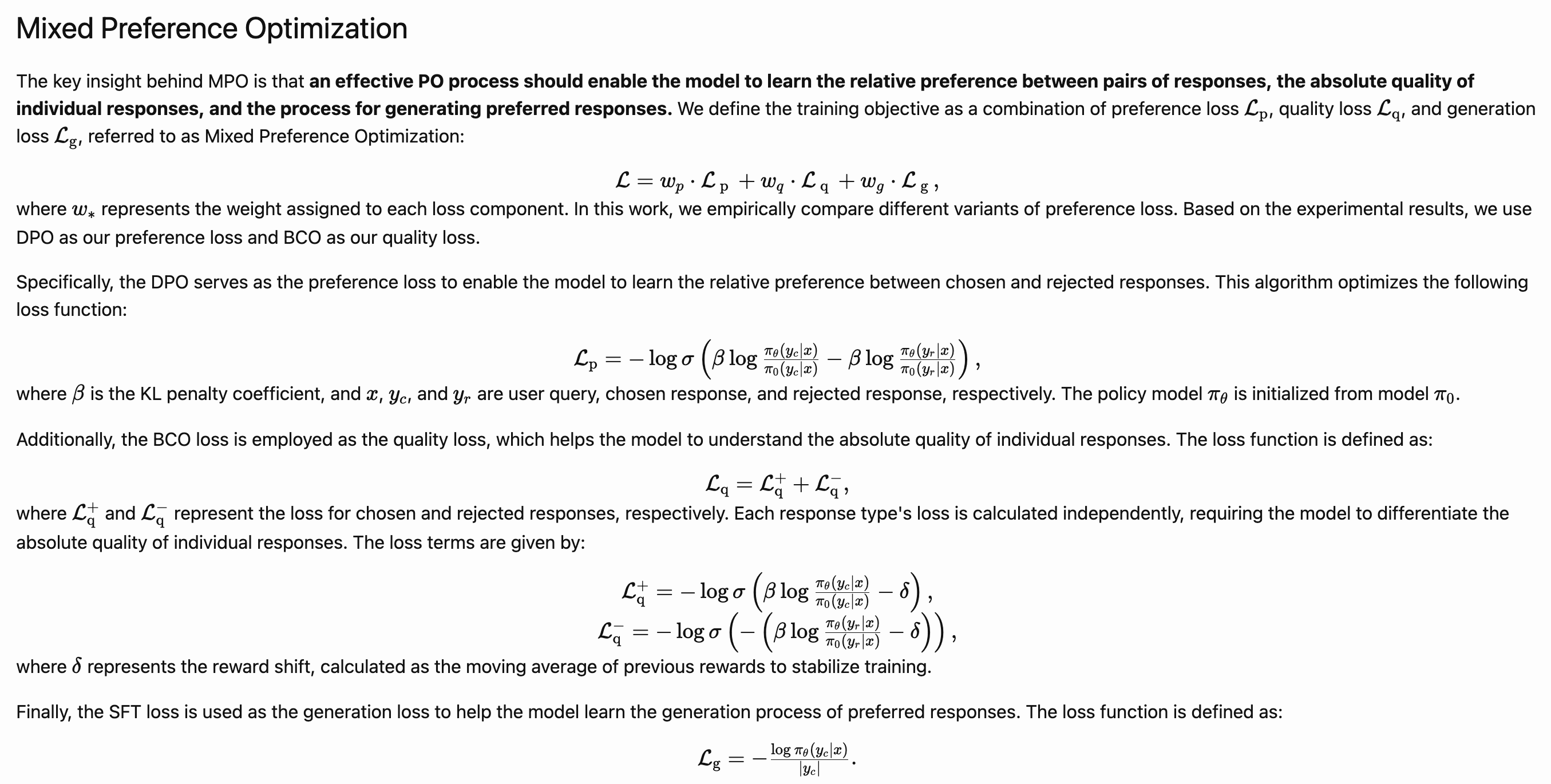
Mixed Preference Optimization

MPO introduces additional supervision from both positive and negative samples to align the model response distribution with the ground-truth distribution, thereby improving reasoning performance.

The training objective of MPO

$$\mathcal{L}=w_{p}\mathcal{L}_{p}+w_{q}\mathcal{L}_{q}+w_{g}\mathcal{L}_{g}$$

is a combination of

• preference loss $\mathcal{L}_{p}$
• quality loss $\mathcal{L}_{q}$
• generation loss $\mathcal{L}_{g}$

Preference loss DPO loss servers as the preference loss to enable the model to learn the relative preference between chosen and rejected responses

$$\mathcal{L}_{p}=-\log\sigma\left( \beta \log \frac{\pi_{\theta}(y_{c}|x)}{\pi_{0}(y_{c}|x)} -\beta \log \frac{\pi_{\theta}(y_{r}|x)}{\pi_{0}(y_{r}|x)} \right)$$

• $\beta$ is the KL penalty coefficient
• the policy model $\pi_{\theta}$ is initialized from model $\pi_{0}$

Quality loss The BCO loss is employed as the quality loss, which helps the model to understand the absolute quality of individual response

$$\mathcal{L}_{q}=\mathcal{L}^+_{q}+\mathcal{L}^-_{q}$$

where $\mathcal{L}^+_{q}$, $\mathcal{L}^-_{q}$ are the loss for the chosen and rejected responses respectively. Calculated independently, requiring the model to differentiate the absolute quality of individual responses.

$$\begin{align} \mathcal{L}^+_{q}&=-\log\sigma\left( \beta \log \frac{\pi_{\theta}(y_{c}|x)}{\pi_{0}(y_{c}|x)}-\delta \right) \\ \mathcal{L}^-_{q}&=-\log\sigma\left( -\left( \beta \log \frac{\pi_{\theta}(y_{r}|x)}{\pi_{0}(y_{r}|x)} -\delta\right) \right) \end{align}$$

• $\delta$ is the reward shift, calculated as the moving average of previous rewards to stabilize training.

Generation loss The LM loss as the generation loss, to help the model learn the process of preferred responses.

$$\mathcal{L}_{\text{text-only}}(\theta)=-\sum_{i=2,~x_{i}\in \text{ Text}}^L w_{i}\cdot \log p_{\theta}(x_{i}|x_{1},\dots,x_{i-1})$$

Test-Time Scaling